SFB 1035 SAXS Instrument

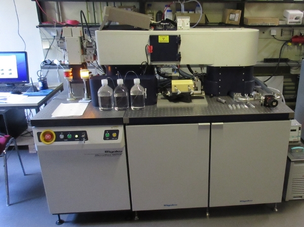
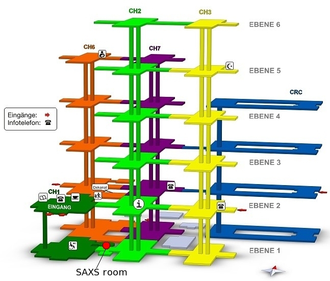
The Rigaku BioSAXS 1000 instrument was purchased by the SFB 1035 as a central service facility. The instrument was installed in August 2013 in Room 11007 in the basement of the chemistry building (green area, room 11007 Tel. 13306). February 2017 the instrument got a new improved autosampler with 96 positions and 6 positions for washing solutions. In summer 2020 the dectris detector was replaced by a new Rigaku HyPix3000 Detector. The optics upgrad to a optiSAXS optics made the instruemnt again to a state of the art bio SAXS instrument.

Measurements

For SAXS measurements please contact Ralf Stehle (ralf.stehle Ät tum.de / 089 289 52613). If you are new to the methode or need help during data evaluation just ask for it. Measuring by yourself is possible too after an introduction into the instrument and radiation protection.

The sample changer has 96 positions. Samples are placed into PCR stripes or plates which are running automatically as a batch. Between the samples and at the begin and end of each batch a buffer measurement is done. Depending on concentration and size of the molecules one measurement needs between 1 and 3 hours.

Samples

• Volume, 70 μl per measurement
• 3 measurements with different concentrations per Sample
• Concentrations:
• Small Proteins: 5-15 mg/ml
• Large Proteins/complexes 1-10 mg/ml
• Keep salt concentration as low as possible but take care that the protein is still stable (better higher salt and low contrast than agglomerates)
• Additives like DTT, TCEP, Thioethanol, Glycerine (up to 5%) reduce beam damage
• buffer is measured before and after each sample, minimum twice so 150 μl or more is needed

Samples should be well characterised before any SAXS measurement. DLS, SLS, GPC (SDS gels alone are not sufficient to prove the quality of a sample). Any impurities specially agglomerates are disturbing the measurement tainting the data processing and results evaluated from the data.

SAXS is highly sensitive to agglomerates. A buffer optimisation for stability is recommended before any measurement is performed. On the other hand SAXS is a senistive tool to test the integrity of a sample and stability in a buffer system.

Frozen samples have to be purified over a size exclusion and reconcentrated very carefully. Upon freezing and thawing of samples some protein molecules form agglomerates which are disturbing measurements and often make data useless.

Salt and additive concentrations have to be exactly the same in the samples and buffers. Do not pipette additives to prepared samples and buffers. Instead prepare the buffer including all additives and then make a solvent exchange with your sample.

Samples prepared from lyophylised material need always a buffer exchange before measurement. Commercially available dried materials contain always salt or stabilising additives which are disturbing the measurement an lead to buffer mismatch.

Complexes of different proteins or protein and RNA/DNA should be prepared in a way that all components are dissolved in the same buffer before mixing. Otherwise a buffer exchange is necessary to keep buffer and sample measurement comparable. Purification over gel filtration after formation of the complex will increase the relaiability of the measurements.

Technical data

X-rays are produced by a Rigaku HF007 microfocus rotating anode with copper as target material. Between kathode and anode 40 kV are accelerating the electrons. The current is 30 mA. The accelerated elecrons push electrons out of the K-shell of copper atoms. Electrons from the L-shell are falling onto the K-shell emmiting characteristic copper Kα x-rays. The Wavelength of these X-rays is 1.54 Angstrom (8 keV). The X-ray beam is focused with a two mirror optics covered with multilayer materials for monocromatisation.

To use more of the solid angle the x-rays are leaving the anode x-rays are focused onto the detector by two perpendicular mirrors. The beam profile is formed by a classical kratky block. Nevertheless due to the optics the rigaku instrument has a point focus saving us from the desmearing during data reduction.

The sample cell is a 1 mm quartz tube with 10 μm wall thickness. This capillary is glued into a steel tube with epoxy and connected to the autosampler via flourinated polymer tubes. Samples are moved with a Hamilton syringe inside the washing station. Relative intensities of samples and tramsmissions are measured by a photodiode beamstop.

The detector is a Rigaku HyPix3000 detector with 100 μm^2 pixel size. In difference to a clasical ccd camera which is read out at the end of a measured frame each photon is counted individually by this detector. This enables the detector to discriminate between x-rays comming from the instrument and photons from cosmic rays or thermal events. The result is a nearly noise free detector image.

The Sample detector distance is 480 mm. A silver behenate sample is mounted on the sample stage of the camera to calibrate the beam center and q-axis at the beginning of each batch.

Primary data is normally measured as multiple 900 second frames which are averaged by the Dectris detector software. The single frames are compared to check for beam damage or air bubbles. Radial averaging and solvent subtraction is done by the Rigaku SAXSLab software. The exported solvent subtracted scattering curves are normalised to concentration and processed further.

Data processing

For data processing beyond the export of solvent subtracted scattering curves the ATSAS package is used. Which version of the package was used for data evaluation depends on the date the calculations were done. Times of usage of special versions is listed below.

Data are stored into a directory structure. The name of the main directory containes the date when the measurement started, a shortcut for the user and a project or protein name.
  Files containing *-info.txt or info-*.txt contain information about the data. transz.txt contains a sumary of measurement parameters, intensities, transmissions, measurement times. A file called info-log.txt or Logbook....html or similar name contains a dump of the measurement logbook. When a file SAXSdatatreatmentlog.html (or similar name) exists a summary of the data treatment is available in a browser readable format.
  Subdirectories:
- raw containes the raw data, detector images in dectris format, measurement schedule in .csv, and an instrument log.... It is a copy of the measurement directory on the instrument.
- export containes the solvent subtracted scattering curves.
- process containes the concentration normalised scattering curves from export. Any further data processing is normally done within this directory.

process:
A table with RG values is called info-RG.txt. If the file does not exist the Rg values are stored in the processing logbook in the main directory. Files with .opj as suffix contain plots of scattering curves and/or pvr data in Microcal Origin format. Plots for publications or reports are taken out from this file.
  Form all scattering curves normaly a fourier transformation is calculated. The output is stored in a .out file. The suffix _a.out means the fourier transformation was donne by the software in auto mode. The suffix _h.out indicates, that the data range, Dmax, alpha-Values were set manually. Files with extracted pvr curves are stored in the subdirectory pvr. One or multiple info-gnom-{date-time}.txt files contain a summary of the output of the fourier transformation in a table.
  With the .out files dummy models are calculated. 10 models are calculated from each file in a subdirectory called work-{date-time}. These models are averaged and filtered. The resulting .pdb files are copied into the subdirectory res-{date-time} with the respective suffix -damfilt.pdb or -damstart.pdb. Often a pymol file *-all.pse containing all calcualted models exist within the res-{date-time} subdirectory. Sometimes it is located directly in process.
  Any further data processing like ensemble or rigid body modeling or fit to crystal data is performed in the subdirectories process/eom, process/coral or process/crysol respectively. Scattering data containing a suffix *_s4.dat are shortened by the indicated number of data points on the low q side. This is necessary to get rid of the data points covered by the beamstop which are disturbing any further calculation.

SAXSLab Versions:

Measurement, Circular averaging, q-calibration, transmission normalisation, solvent subtraction, and export to 1D-files is done with this software:
SAXSLab 2.0.0b23 up to 12.8.2013
SAXSLab 2.0.0b26 from 12.8.2013 to 23.9.2013
SAXSLab 3.0.0r1 from 23.9.2013 to 16.10.2013
SAXSLab 3.0.1r1 from 16.10.2013 to 17.10.2013
SAXSLab 3.0.0r1 from 17.10.2013 to 11.2.2014
SAXSLab 3.0.2b7 from 11.2.2014 to 5.5.2014
SAXSLab 3.0.2 from 5.5.2014 to 11.7.2014
SAXSLab 3.0.2new070714 from 11.7.2014 to 16.1.2017 (bugfix release directly from the software developers)
SAXSLab 3.1.0 from 16.1.2017 to 16.6.2020
SAXSLab 3.1.1 from 18.6.2020


ATSAS Versions:
Data treatment is done with different ATSAS Versions, depending on when the treatment was done the version is:
ATSAS 2.5.0 from 2013 to 16.5.15
ATSAS 2.6.0 from 16.5.15 to 14.10.15
ATSAS 2.7.0 from 14.10.15 to 11.1.17
ATSAS 2.8.0 from 11.1.16 to 12.12.17
ATSAS 2.8.3 from 12.12.17 to 7.12.19
ATSAS 3.0.0 from 07.12.19

The ATSAS package is available at the EMBL in Hamburg for free (registration necessary).

SASView:
SasView 4.1.2 up to 19.3.2019
SasView 4.2.1 from 19.3.2019

Responsibilities

• Responsible for the instrument: Ralf Stehle (room 32201, phone 13305)
• Local radiation Protection: Ralf Stehle, Michael Groll (room 32201, phone 13305. room 52311 phone 13361)
• Radiation protection TUM: Peter Sabath, Fr Rauh (HR6, phone 14680. phone 14678)
• SAXS room 11007 (Tel. 13306)

Text

common text blocks for reports and publications:

       SAXS measurements were carried out on a Rigaku BioSAXS1000 instrument with a HF007 
       microfocus copper target (40 kV, 30 mA) an optiSAXS optics and a HyPix3000 detector. 
       For q calibration a silver behenate sample (Alpha Aeser) was used. Transmissions were 
       measured with a photodiode beamstop. Samples were measured in 4/8 900 second frames 
       checked for beam damage, circular averaged and solvent subtracted by the SAXSLab 
       software (v 3.1.1). Three concentrations ( x,y,z mg/ml) were measured from each sample normalized 
       to concentration and compared to exclude concentration dependent effects..... 
       
       Pair distance distributions, low resolution Models, and rigid body models were calculated with the ATSAS package v2.5.0.2/2.7.0.1. 
       Molecular weights were calculated from Porod Volume.         
       

       .....we aknowledge the SFB 1035 for SAXS measurements.....
       

If SasView is used the authors of the software recommend the following aknowledgement:

      
        This work benefited from the use of the SasView application, originally developed under NSF Award DMR-0520547. 
        SasView also contains code developed with funding from the EU Horizon 2020 programme under the SINE2020 project Grant No 654000.
       

Literature

A comprehensive introduction in scattering methods:
Neutron X-rays and Light: Scattering Methods Applied to Soft Condensed Matter
Peter Lindner, Th. Zemb (Elsevier, 2002, ISBN-10: 0444511229)

Chapter 3 gives a good introduction into scattering theory.
Chapter 4 describes scattering theory a bit different and adds some detais.
Chapter 2 deals more with practical aspects of scattering data and theory.
Chapter 5 specialises on the fourier transformation and pair distance distribution function.

A bit more detailed and a lot more mathematical the book of Guinier and Fournet:
Small-Angle Scattering of X-rays
A. Guinier, G. Fournet (Wiley, 1955, sometimes available as scan on the internet)

Overview over the ATSAS package:
New developments in the ATSAS program package for small-angle scattering data analysis
Petoukhov, M. V.; Franke, D.; Shkumatov, A. V.; Tria, G.; Kikhney, A. G.; Gajda, M.; Gorba, C.; Mertens, H. D. T.; Konarev, P. V., Svergun, D. I. (Journal of Applied Crystallography, International Union of Crystallography, 2012, 45, 342-350)
doi:10.1107/S0021889812007662

SasView 4.2.1:
M. Doucet, et al. SasView Version 4.2.1 http://doi.org/10.5281/zenodo.2561236

An online course for powder diffraction explaines the basics of x-ray production and scattering theory:
Powder diffraction course

SAS course

A training course in small angle scattering for doctoral students and postdocs is held once a year. This course shows the scattering theory briefly and focuses more on measurement and data evaluation. One main part of the course are practical exercises in data evaluation.

Next SAS course will be 4-6.3.2020
Programm 2020

SAXS course 28.3.2019 BNMRZ seminar room:
Programm 2019
Introduction
Basic data evaluation

Handouts of the course december 2017:
Programm 2017
Introduction to SAXS, theory and sample preparation
Overview of basic data evaluation and analysis

Radiation protection

People who want to run the instrument by their own need an introduction into the instrument handling and a safety introduction into radiation protection which has to be repeated yearly.

Other Stuff concerning safety and radition protection:
Radiation protection instruction
Emergency ToDo List
Alarming List
Safety Instruction
Emergency telefon number list

Strahlenschutz Gesetz
Strahlenschutz Verordnung